PyCaret Tutorial

PyCaret Tutorial

This tutorial will not cover PyCaret as a whole, but it will rather focus on the entire pipeline for a single classification problem. We will use the wine recognition dataset:

Lichman, M. (2013). UCI Machine Learning Repository. Irvine, CA: University of California, School of Information and Computer Science.

OBS: This post was automatically generated from my Jupyter Notebook thanks to Adam Blomberg’s post.

What is PyCaret?

PyCaret is a library that comes to automate the Machine Learning (ML) process requiring very few lines of code. It works with multiple other useful ML libraries, such as scikit-learn.

Check out their website for more information: PyCaret Homepage.

Installing PyCaret

Virtual environment

First, we create a virtual environment to ensure we do not have unnecessary packages as well as to keep things isolated and light.

Using venv:

$ python -m venv /path/to/new/virtual/environment

And to activate it:

$ source /path/to/new/virtual/environment/bin activate

Using conda:

$ conda create --name venv pip

And to activate it:

$ conda source venv activate

Actual PyCaret installation

We use pip to install it:

$ pip install pycaret

Or on the notebook:

! pip install pycaret

Dataset

We will import the dataset from Scikit-learn:

import sklearn
from sklearn.datasets import load_wine
print(f"Scikit-learn version: {sklearn.__version__}")
import pandas as pd
import numpy as np

Scikit-learn version: 0.23.2

data = load_wine()
df = pd.DataFrame(data=np.c_[data['data'], data['target']],
                  columns=data['feature_names'] + ['target'])
df.shape

(178, 14)

Let’s do some very brief EDA on the dataset:

display(df.head())
df.describe()

	alcohol	malic_acid	ash	alcalinity_of_ash	magnesium	total_phenols	flavanoids	nonflavanoid_phenols	proanthocyanins	color_intensity	hue	od280/od315_of_diluted_wines	proline	target
0	14.23	1.71	2.43	15.6	127.0	2.80	3.06	0.28	2.29	5.64	1.04	3.92	1065.0	0.0
1	13.20	1.78	2.14	11.2	100.0	2.65	2.76	0.26	1.28	4.38	1.05	3.40	1050.0	0.0
2	13.16	2.36	2.67	18.6	101.0	2.80	3.24	0.30	2.81	5.68	1.03	3.17	1185.0	0.0
3	14.37	1.95	2.50	16.8	113.0	3.85	3.49	0.24	2.18	7.80	0.86	3.45	1480.0	0.0
4	13.24	2.59	2.87	21.0	118.0	2.80	2.69	0.39	1.82	4.32	1.04	2.93	735.0	0.0

	alcohol	malic_acid	ash	alcalinity_of_ash	magnesium	total_phenols	flavanoids	nonflavanoid_phenols	proanthocyanins	color_intensity	hue	od280/od315_of_diluted_wines	proline	target
count	178.000000	178.000000	178.000000	178.000000	178.000000	178.000000	178.000000	178.000000	178.000000	178.000000	178.000000	178.000000	178.000000	178.000000
mean	13.000618	2.336348	2.366517	19.494944	99.741573	2.295112	2.029270	0.361854	1.590899	5.058090	0.957449	2.611685	746.893258	0.938202
std	0.811827	1.117146	0.274344	3.339564	14.282484	0.625851	0.998859	0.124453	0.572359	2.318286	0.228572	0.709990	314.907474	0.775035
min	11.030000	0.740000	1.360000	10.600000	70.000000	0.980000	0.340000	0.130000	0.410000	1.280000	0.480000	1.270000	278.000000	0.000000
25%	12.362500	1.602500	2.210000	17.200000	88.000000	1.742500	1.205000	0.270000	1.250000	3.220000	0.782500	1.937500	500.500000	0.000000
50%	13.050000	1.865000	2.360000	19.500000	98.000000	2.355000	2.135000	0.340000	1.555000	4.690000	0.965000	2.780000	673.500000	1.000000
75%	13.677500	3.082500	2.557500	21.500000	107.000000	2.800000	2.875000	0.437500	1.950000	6.200000	1.120000	3.170000	985.000000	2.000000
max	14.830000	5.800000	3.230000	30.000000	162.000000	3.880000	5.080000	0.660000	3.580000	13.000000	1.710000	4.000000	1680.000000	2.000000

All data is numeric and without missing values.

# Checking the classes
df['target'].value_counts()

1.0    71
0.0    59
2.0    48
Name: target, dtype: int64

The classes are not very imbalanced.

Splitting the dataset into train and test

from sklearn.model_selection import train_test_split

df_train, df_test = train_test_split(df,
                                     test_size=0.20,
                                     random_state=0,
                                     stratify=df['target'])

Initializing PyCaret

We can, now, import PyCaret and start playing around with it!

import pycaret
from pycaret.classification import *
print(f"PyCaret version: {pycaret.__version__}")

PyCaret version: 2.3.1

PyCaret syntax asks us to setup the data as the first step, providing the input data with the features and the target variable. This setup function is how PyCaret initializes the pipeline for future preprocessing, modeling, and deployment. It requires two parameters: data, a pandas dataframe, and target, the name of the target column. There are other parameters, but they are all optional and we will not cover them at this point.

The setup infers on its own the features’ data types, but it is worth double checking since it may do it incorrectly sometimes. A table showing the features and their data types is displayed after running the setup. It asks us to confirm if correct and press enter. If something is incorrect, then we can correct it by typing quit. Otherwise, we can proceed. Notice that getting the data types right is extremely important, because PyCaret automatically preprocesses the data based on each feature’s type. Preprocessing is a fundamental and critical part of doing ML properly.

# setup the dataset
grid = setup(data=df_train, target='target')

	Description	Value
0	session_id	6420
1	Target	target
2	Target Type	Multiclass
3	Label Encoded	None
4	Original Data	(142, 14)
5	Missing Values	False
6	Numeric Features	13
7	Categorical Features	0
8	Ordinal Features	False
9	High Cardinality Features	False
10	High Cardinality Method	None
11	Transformed Train Set	(99, 13)
12	Transformed Test Set	(43, 13)
13	Shuffle Train-Test	True
14	Stratify Train-Test	False
15	Fold Generator	StratifiedKFold
16	Fold Number	10
17	CPU Jobs	-1
18	Use GPU	False
19	Log Experiment	False
20	Experiment Name	clf-default-name
21	USI	6d1b
22	Imputation Type	simple
23	Iterative Imputation Iteration	None
24	Numeric Imputer	mean
25	Iterative Imputation Numeric Model	None
26	Categorical Imputer	constant
27	Iterative Imputation Categorical Model	None
28	Unknown Categoricals Handling	least_frequent
29	Normalize	False
30	Normalize Method	None
31	Transformation	False
32	Transformation Method	None
33	PCA	False
34	PCA Method	None
35	PCA Components	None
36	Ignore Low Variance	False
37	Combine Rare Levels	False
38	Rare Level Threshold	None
39	Numeric Binning	False
40	Remove Outliers	False
41	Outliers Threshold	None
42	Remove Multicollinearity	False
43	Multicollinearity Threshold	None
44	Clustering	False
45	Clustering Iteration	None
46	Polynomial Features	False
47	Polynomial Degree	None
48	Trignometry Features	False
49	Polynomial Threshold	None
50	Group Features	False
51	Feature Selection	False
52	Feature Selection Method	classic
53	Features Selection Threshold	None
54	Feature Interaction	False
55	Feature Ratio	False
56	Interaction Threshold	None
57	Fix Imbalance	False
58	Fix Imbalance Method	SMOTE

Among the optional parameters we skipped, there were options for preprocessing such as outline removal, feature selection, feature encoding, dimensionality reduction, how to split between train and test set, and many more! Check out the documentation for more details.

Comparing different models

After setting up, the time to compare and evaluate different models has arrived! And this is done so easily that pretty much anyone with a minimal knowledge on metrics could pick up the best model. This is one of the cool PyCaret’s features that allows us to save a lot of time.

PyCaret uses 10-fold cross-validation as its default, sort results by classification accuracy, returns the best model, and displays the results of all tested classifiers with different metrics.

best = compare_models()

	Model	Accuracy	AUC	Recall	Prec.	F1	Kappa	MCC	TT (Sec)
rf	Random Forest Classifier	0.9700	0.9975	0.9750	0.9770	0.9698	0.9545	0.9585	0.0790
nb	Naive Bayes	0.9600	0.9950	0.9639	0.9678	0.9598	0.9394	0.9431	0.0060
et	Extra Trees Classifier	0.9600	0.9967	0.9700	0.9703	0.9604	0.9384	0.9438	0.0670
ridge	Ridge Classifier	0.9589	0.0000	0.9600	0.9686	0.9578	0.9365	0.9423	0.0050
lightgbm	Light Gradient Boosting Machine	0.9500	1.0000	0.9589	0.9623	0.9486	0.9242	0.9315	0.1100
lda	Linear Discriminant Analysis	0.9489	0.9936	0.9533	0.9619	0.9483	0.9211	0.9283	0.0060
qda	Quadratic Discriminant Analysis	0.9389	0.9950	0.9167	0.9534	0.9319	0.9023	0.9135	0.0070
dt	Decision Tree Classifier	0.9200	0.9369	0.9167	0.9330	0.9178	0.8773	0.8855	0.0060
lr	Logistic Regression	0.9189	0.9888	0.9194	0.9314	0.9175	0.8762	0.8830	0.4420
gbc	Gradient Boosting Classifier	0.8900	0.9876	0.8922	0.9127	0.8883	0.8290	0.8416	0.0770
ada	Ada Boost Classifier	0.8489	0.9378	0.8378	0.8721	0.8440	0.7652	0.7782	0.0320
knn	K Neighbors Classifier	0.7178	0.8830	0.6922	0.7521	0.7012	0.5651	0.5915	0.0090
svm	SVM - Linear Kernel	0.5978	0.0000	0.5678	0.5420	0.5152	0.3702	0.4458	0.0070

Showing the best classifier:

print(best)

RandomForestClassifier(bootstrap=True, ccp_alpha=0.0, class_weight=None,
                       criterion='gini', max_depth=None, max_features='auto',
                       max_leaf_nodes=None, max_samples=None,
                       min_impurity_decrease=0.0, min_impurity_split=None,
                       min_samples_leaf=1, min_samples_split=2,
                       min_weight_fraction_leaf=0.0, n_estimators=100,
                       n_jobs=-1, oob_score=False, random_state=6420, verbose=0,
                       warm_start=False)

Tuning a model

The models used when comparing use their default hyperparameters. We can tune and choose the best hyperparameters for a single model using PyCaret. This is done by running a Random Grid Search on a specific search space. We can, as well, define a custom search grid, but we will not do it at this point. Also, there are many hyperparameters that allow us to choose early stopping, number of iterations, which metric to optimize for, and so on. Tuning returns a similar table as before, but each row now shows the result for each validation fold.

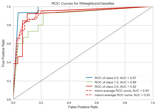
We will tune the K Neighbors Classifier, since it performed poorly with its default parameters. To do so, we first create a model with PyCaret:

from sklearn.neighbors import KNeighborsClassifier

tuned_knn = tune_model(KNeighborsClassifier(), n_iter=100)

	Accuracy	AUC	Recall	Prec.	F1	Kappa	MCC
0	1.0000	1.0000	1.0000	1.0000	1.0000	1.0000	1.0000
1	0.9000	0.9300	0.9333	0.9250	0.9016	0.8438	0.8573
2	0.7000	0.7929	0.6944	0.7400	0.7067	0.5385	0.5471
3	0.8000	0.9083	0.8056	0.8250	0.7971	0.6970	0.7078
4	0.9000	0.9012	0.8889	0.9200	0.8956	0.8462	0.8598
5	0.8000	0.8298	0.7778	0.8450	0.7627	0.6923	0.7273
6	0.7000	0.8857	0.6944	0.7400	0.7067	0.5385	0.5471
7	0.9000	1.0000	0.9167	0.9333	0.9029	0.8485	0.8616
8	0.8000	0.8458	0.8333	0.9000	0.8000	0.7059	0.7500
9	0.7778	0.9000	0.6667	0.6296	0.6889	0.6250	0.6934
Mean	0.8278	0.8994	0.8211	0.8458	0.8162	0.7335	0.7551
SD	0.0910	0.0637	0.1079	0.1076	0.0993	0.1417	0.1364

print(tuned_knn)

KNeighborsClassifier(algorithm='auto', leaf_size=30, metric='manhattan',
                     metric_params=None, n_jobs=None, n_neighbors=3, p=2,
                     weights='distance')

Plotting a model

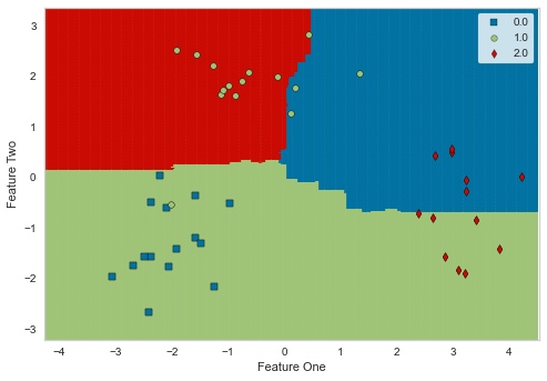
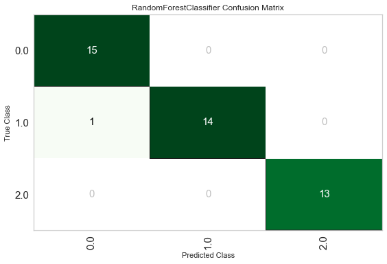
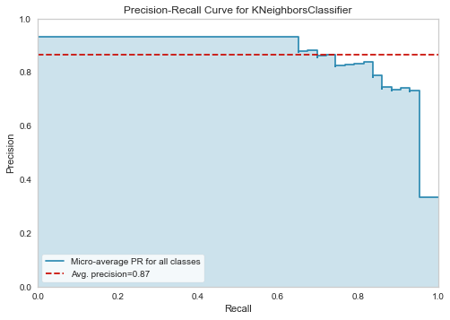
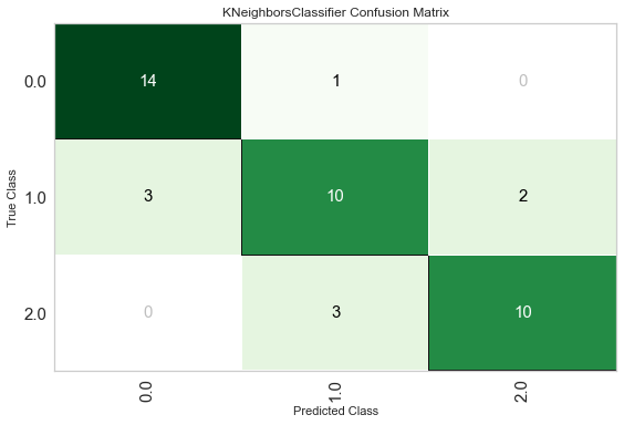
If just seeing a table is not enough, you can plot the results of a model in different ways. Here are a few examples:

plot_model(best, plot='boundary')

plot_model(best, plot='confusion_matrix')

plot_model(tuned_knn, plot='pr')

plot_model(tuned_knn, plot='class_report')

plot_model(tuned_knn, plot='confusion_matrix')

plot_model(tuned_knn, plot='auc')

Explainable AI

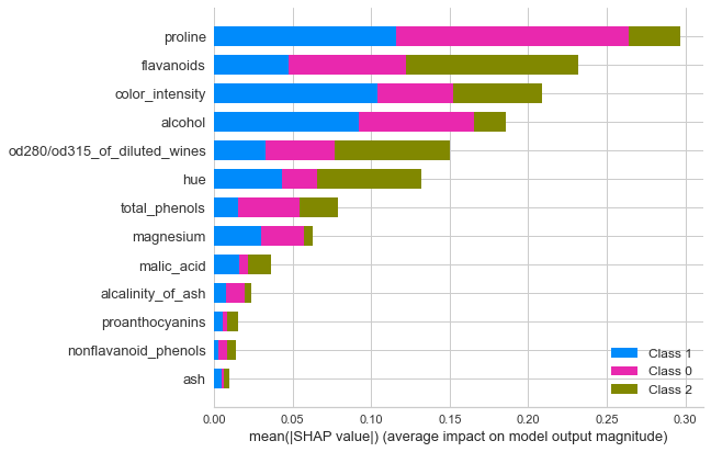
Most businesses do not like to have a black-box model telling them what to do. It is extremely important to understand what the model does so that the business can take action to improve their results.

For this, we need to install the shap library:

$ pip install shap

Or on the notebook:

! pip install shap

This library is based on the concept of Shapley values created in the Game Theory context to compute feature importance. For now, it is only available for tree-based models.

from sklearn.ensemble import RandomForestClassifier
rf = create_model(RandomForestClassifier())

	Accuracy	AUC	Recall	Prec.	F1	Kappa	MCC
0	1.0000	1.0000	1.0000	1.0000	1.0000	1.0000	1.0000
1	1.0000	1.0000	1.0000	1.0000	1.0000	1.0000	1.0000
2	1.0000	1.0000	1.0000	1.0000	1.0000	1.0000	1.0000
3	0.9000	1.0000	0.9167	0.9250	0.9000	0.8507	0.8636
4	1.0000	1.0000	1.0000	1.0000	1.0000	1.0000	1.0000
5	0.9000	1.0000	0.9167	0.9250	0.9000	0.8507	0.8636
6	1.0000	1.0000	1.0000	1.0000	1.0000	1.0000	1.0000
7	0.9000	0.9667	0.9167	0.9200	0.8984	0.8438	0.8573
8	1.0000	1.0000	1.0000	1.0000	1.0000	1.0000	1.0000
9	1.0000	1.0000	1.0000	1.0000	1.0000	1.0000	1.0000
Mean	0.9700	0.9967	0.9750	0.9770	0.9698	0.9545	0.9585
SD	0.0458	0.0100	0.0382	0.0352	0.0461	0.0695	0.0635

Summary plot

interpret_model(rf, plot='summary')

Correlation plot

interpret_model(rf, plot='correlation')

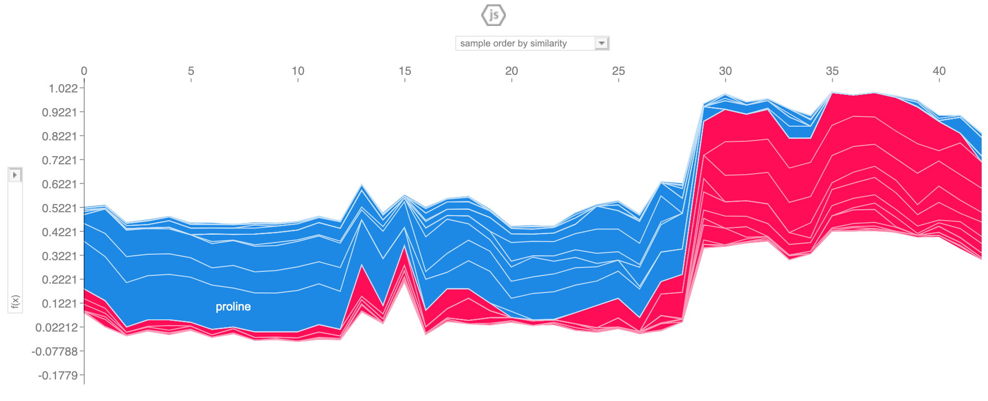
Reason plot

All observation

interpret_model(rf, plot='reason')

A specific observation

interpret_model(rf, plot='reason', observation=10)

Predicting

Now that the exploratory phase is over, we can predict the results on unseen data.

best_final = finalize_model(best)
predictions = predict_model(best_final, data=df_test.drop('target', axis=1))

from sklearn.metrics import classification_report

print(classification_report(df_test['target'], predictions['Label']))

              precision    recall  f1-score   support

         0.0       1.00      1.00      1.00        12
         1.0       1.00      1.00      1.00        14
         2.0       1.00      1.00      1.00        10

    accuracy                           1.00        36
   macro avg       1.00      1.00      1.00        36
weighted avg       1.00      1.00      1.00        36

What now?

PyCaret allows you to do predictions direct from the cloud, so check it out in their website if you want to do this.

Also, you can build your ensemble models with PyCaret.

They support not only Classification, but also Regression, Anomaly Detection, Clustering, Natural Language Processing, and Association Rules Mining.

References

[1] PyCaret Homepage

[2] PyCaret documentation

[3] Multiclass Classification Tutorial

[4] A Gentle Introduction to PyCaret for Machine Learning